Minimalist ESF, LSF, MTF by Monotonic Regression

Because the Slanted Edge Method of estimating the Spectral Frequency Response of a camera and lens is one of the more popular articles on this site, I have fielded variations on the following question many times over the past ten years:

How do you go from the intensity cloud produced by the projection of a slanted edge captured in a raw file to a good estimate of the relevant Line Spread Function?

Figure 1. Slanted edge captured in the raw data and projected to the edge normal. The data noisy because of shot noise and PRNU. How to estimate the underlying edge profile (orange line, the Edge Spread Function)?

So I decided to write down the answer that I have settled on. It relies on monotone spline regression to obtain an Edge Spread Function (ESF) and then reuses the parameters of the regression to infer the relative regularized Line Spread Function (LSF) analytically in one go.

This front-loads all uncertainty to just the estimation of the ESF since the other steps on the way to the SFR become purely mechanical. In addition the monotonicity constraint puts some guardrails around the curve, keeping it on the straight and narrow without further effort.

This minimalist, what-you-see-is-what-you-get approach gets around the usual need for signal conditioning such as binning, finite difference calculations and other filtering, with their drawbacks and compensations. It has the potential to be further refined so consider it a hot-rod DIY kit. Even so it is an intuitively direct implementation of the method and it provides strong validation for Frans van den Bergh’s open source MTF Mapper, the undisputed king in this space,^[1] as it produces very similar results with raw slanted edge captures.

I expect this article to only be of interest to keen imaging nerds so I will dive right in, presuming familiarity with the preliminaries, which were partly covered in the article up top. If you come up with some refinement or spot some weaknesses let me know, I am interested as always.

The Slanted Edge Method in a Nutshell

The slanted edge method aims to estimate the Modulation Transfer Function (a.k.a SFR) of an imaging system by capturing slanted edges in a raw file. The procedure is simple in principle: capture with good technique the image of an edge in the raw data with a monochrome or Bayer image sensor, subtract the black-level and estimate the angle of the edge accurately so that the two-dimensional pixel grid can be projected onto a one-dimensional edge normal.

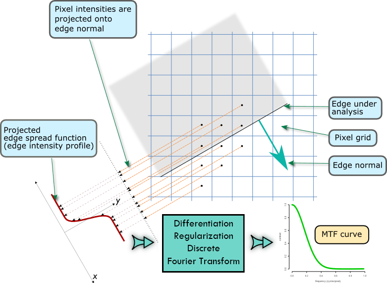
Figure 2. Pixel grid projected to edge normal with relative pixel intensities, the Edge Spread Function. Differentiation results in a Line Spread Function, which after regularization and Fast Fourier Transformation produces the Modulation Transfer Function of the imaging system in the center of the edge in the direction perpendicular to it. Image courtesy of Frans van den Bergh, modified to reflect article variables.

The result is a set of data pairs ( $x_i,y_i$ ), with $x_i$ representing the exact position on the normal axis and $y_i$ the (noisy) intensity of the projected pixel.

If the sensor comes with a Bayer Color Filter Array we may elect to use data pairs from a given color channel only, obtaining results for the respective $r$ , $g$ and/or $b$ raw plane separately; or white balance the raw data as-is and effectively end up with a full-resolution monochrome capture representing the performance of the $rgb$ system as a whole. The latter produces a weighted average of the results of the former.

Either way, once sorted based on $x$ and plotted, the data pairs typically appear at non-uniform intervals on the normal axis and look something similar to Figure 1. They represent a super-sampled, noisy, intensity profile of the edge. The underlying edge profile curve is then

estimated as the so-called Edge Spread Function;
regularized; and
differentiated to obtain the relative Line Spread Function,

2 and 3 not necessarily in that order. This article is mainly about these three critical steps.

Finally the LSF is put through a Discrete Fourier Transform routine to produce its Spectral Frequency Response which, with a good target like a back-lit knife edge, represents the Modulation Transfer Function (MTF) of the imaging system, at the center of the edge in the direction perpendicular to it.

Why Monotonic?

The short answer is that theoretically the LSF is just a projection to one dimension of the normalized impulse response of the system, the two dimensional Point Spread Function, which is by definition made up of only non-negative intensity. Therefore the Line Spread Function is also non-negative and so is the ESF, its running integral.

Figure 3. Left: PSF of a typical imaging system with square pixels, an antialiasing filter and a lens at f/4. Center: LSF, same intensities as PSF but projected on the edge normal. Right: ESF, cumulative sum of LSF left to right.

As the cumulative sum of the LSF moves along its axis it should only find non-negative numbers to add up so the resulting ESF curve should only increase or stay the same at each subsequent step.

Therefore ideally the physical profile of the edge from a linear raw file is always monotonic (a.k.a. isotonic) as clearly seen in the trend in the Figures in this page,^[*] a fact that we should be able to rely on and exploit to our advantage to produce a more robust and better behaved curve, as will be discussed further down.

Processing such as sharpening and some demosaicing can induce over and undershoots in the ESF so monotonicity is only guaranteed in the case of linear raw data, which is solely what this article and these pages are concerned with. Not to worry though, the minimalist approach can also be used to produce non-monotonic ESFs, losing the monotonic guardrails but still maintaining its other advantages.

Noisy, Noisy

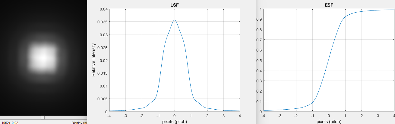
Data Numbers of captured raw intensity are not monotonic when projected onto the edge normal because they are noisy. In testing conditions sources of noise are mainly shot noise and Pixel Response Non Uniformities, both of which increase with intensity, the reason why the dark portion of the projected edge looks less noisy than the bright one in Figure 1.

Figure 4. Raw intensities projected on the edge normal are not monotonic mainly because of shot noise and Pixel Response non Uniformities. Snippet of projected data about 16 pixels to the left of the edge.

This is a problem because in order to obtain the MTF curve we need to differentiate and regularize the projected raw data to obtain a LSF to feed to a Fast Fourier Transform routine. Differentiation amplifies noise. It is usually implemented as finite differences of the ( $x_i,y_i$ ) raw data pairs, making unconditioned projected raw edge data unusable for this purpose in virtually all circumstances. Below you can see a brute force application of finite differences to the full set of projected raw edge data around the transition:

Figure 5. What happens if you differentiate the data in Figure 1 by finite difference.

So how best to tease out the monotonic edge profile curve hiding in the noise, nuances and all? Folks early in the journey, including younger me, often assume that the ESF or the LSF are only made up of well behaved shapes like sigmoids or gaussians and presume that’s what’s behind the noise. However, differences from simple shapes is where high frequency detail resides so with that assumption we are giving up accuracy and throwing out a meaningful portion of the spectrum unnecessarily.

In photography we are often interested in those higher frequencies because they can provide a measure of the physical characteristics and capabilities of the imaging system, such as lens working f-number, the size of effective pixel aperture, the presence of antialiasing or other filtering. Horses for courses.

The Naive Approach

One intuitive solution often seen in the literature is to average the projected raw intensities, say every quarter or eighth of a pixel. This does regularize the data while providing some noise reduction, though it is equivalent to convolving the raw capture of the edge with a weirdly shaped filter, changing the underlying data and smoothing the Edge Spread Function, hence the apparent frequency response of the imaging system.

Differentiation to obtain the LSF is then usually computed by finite difference, another operation which effectively filters the data, this time amplifying noise. Since the two filtering functions above are known, their effect can be partly reversed in the frequency domain, and that’s what the naive approach does, see for instance this Peter Burns paper.^[2]

There is no free lunch however, so while the MTF may be compensated for before display, the incorrectly smoothed and sharpened LSF is abandoned as such, starving the higher frequencies of energy thus driving them into the noise.

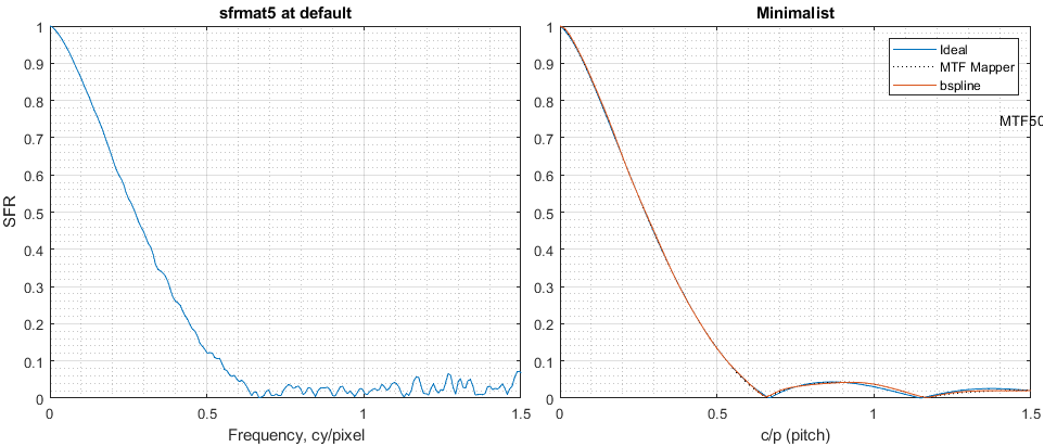
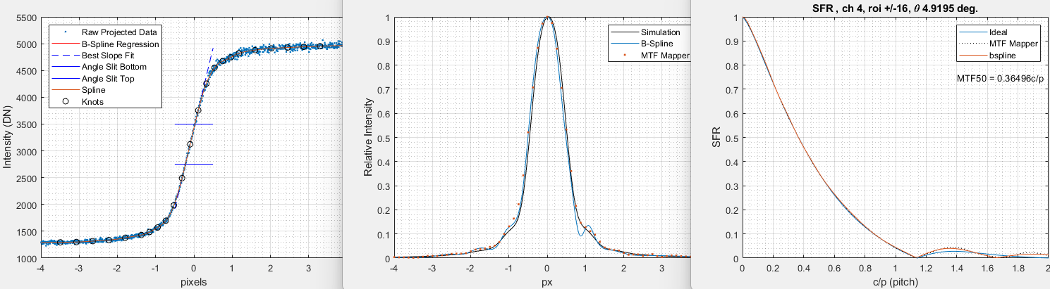
Too bad, because there is often neat information to be gleaned there. Below left the naive approach is represented by the ISO12233 v4 2023 algorithm at default: it understates MTF and misses the AA and pixel aperture nulls at 2/3 c/p and 1.143 c/p respectively.^[3] The minimalist approach to the right instead follows the theoretical MTF curve almost perfectly – as does our reference, MTF Mapper 0.7.40.

Figure 6. MTF from theoretically accurate, noisy slanted edge captured in the raw data by a monochrome sensor with the noise characteristics of a FF MILC camera, known pixel aperture null at 1.143 c/p and antialiasing filter null at 2/3 c/p, with a 24mm lens at f/4. The ideal PSF, LSF and ESF are those shown in Figure 3.

In addition, the naive approach does not result in a physically correct, monotonic ESF therefore it can wander off the beaten path, losing sensitivity and detail. It is also forced to compensate for the data conditioning that it needs to perform, potentially introducing biases along the way (see comment by reader Larry a while back).

Why Regression

Regression fits the bill because it can answer questions like this: given the entire set of data in Figure 1, what is the one curve most likely to minimize squared deviations from it, subject to a set of given conditions?

The uncertainty here is only in the intensities ( $y_i$ ) while the independent variable representing the position of the relative pixels ( $x_i$ ) can be considered to be known exactly so the least squares minimization criterion is relevant (vs. orthogonal for instance). It also helps that the dominant source of noise, shot noise, induces intensity swings proportional to the square root of the mean photoelectron signal.

Monotonicity is just an additional constraint put on the regression. My first attempt at generating an ESF by monotonic regression worked but was cumbersome and it took a quarter of an hour to compute with a typical edge. I mentioned this to Frans van den Bergh who quickly found a lightening fast C implementation of it by Dr. Jan de Leeuw based on J.B. Kruskal’s Pool Adjacent Violators algorithm (PAVA, 1964).^[4]

The Pool-Adjacent-Violators-Algorithm

Dr. de Leeuw is the Distinguished Professor of Statistics and former chairperson of the Department of Data Theory at Leiden University. With Frans’ help I was able to make the jbkpava.c routine in his paper play nice with Matlab. However, it turns out that Matlab has its own open domain version of it, lsqisotonic,^[5] so suddenly I could generate monotonic ESFs from projected raw edge intensity data pairs in microseconds.

Figure 7. Kruskal’s Pool-Adjacent-Violators Algorithm regression provides a good first approximation to the ESF. But the stair-stepping creates harmonics which result in high frequency noise.

As you can see in the Figure above results are pretty good when seen at scale but the algorithm produces jumps from one monotone level to the next, introducing stair-stepping in the curve. Even though they can be considered micro-steps because of how frequent they are, they generate harmonics resulting in a noisier response at higher frequencies.

An additional issue is that the resulting PAVA ESF produces a regressed $\hat y_i$ data point at each originally scattered $x_i$ so the data still needs to be differentiated and regularized in order to be fed to the Fast Fourier Transform routine. This is easiest done by filtering equivalent to – you guessed it – binning, which partly defeats the purpose because it results in another version of the sharpness-reduced and noise-increased LSF of the naive approach, only uglier.

Nevertheless the PAVA regressed ESF is indeed monotonic and as such better behaved than most. If you bin it, say, every eighth or quarter of a pixel and compensate for it and the finite difference subtraction in the frequency domain, the resulting MTF turns out to be better than the vast majority of algorithms out there on raw data.

For example in the Figure below PAVA is more accurate, less noisy, and capable of showing the Nikon Z7’s pixel aperture null estimated at around 1.15 c/p – compared to sfrmat5 at default,^[3] which appears to underestimate MTF throughout and loses the null in the noise.

Figure 8. MTF from Slanted edge captured in the center of the raw file of a Nikon Z7 with 24-70/4 S lens at 24mm, f/5.6, white balanced and fed as a grayscale image to both sfrmat5 at default (left) and the described PAVA algorithm (right).

So how to avoid the stepping, binning and differentiating problems?

Splines to the Rescue

With some time on my hands during Covid I contacted Dr. de Leeuw for a solution to the stair-stepping issue. He suggested I take a look at his work on monotonic spline regression. I did – and never looked back.

The idea behind splines in our context is to break down the pixel axis in Figure 1 into arbitrary sequential segments and fit the projected raw intensity data [ $x_i,y_i$ ) within each segment with a polynomial of a chosen degree in such a way that the curve generated in each segment is continuous with its neighbors.

Figure 9. Top: cubic splines; bottom: the relative spline function, courtesy of Mathworks.

I am taking a few liberties with the narrative for simplicity here, refer to Dr. de Leeuw’s ‘Computing and Fitting Montone Splines‘ working paper for the correct level of detail in this explanation.^[6] As a reminder a, say, cubic polynomial has this form:

(1) $\begin{equation*} \begin{align} \left f(x) \right &= ax^3+bx^2+cx+d \\ \\ &= \begin{bmatrix} x^3 & x^2 & x & 1 \end{bmatrix} \left[\begin{array}{c} a \\ b \\ c \\ d \end{array}\right] \\ &= h*u \end{align} \end{equation*}$

with $a$ not zero and $x$ the horizontal axis. The formula in the middle is the same as the one at the top but in matrix notation, which simplifies reading and following the code in the notes. The first term on the right hand side collects the basis functions, call them $h$ , while the second the coefficients, call them $u$ , with matrix multiplication indicated by the $*$ character.

The highest exponent determines the degree of the polynomial, in this example it is 3. The idea is to use regression within each segment to find the $[a,b,c,...]$ coefficients that best match the $[x_i,y_i)$ data by least squares using a monotonicity constraint.

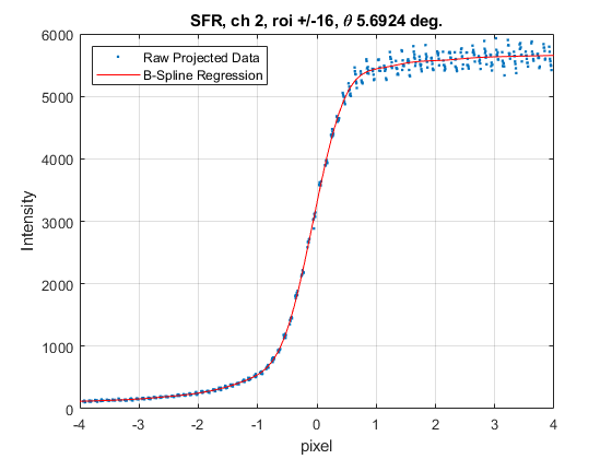
The resulting curve spanning the entire data set is called a spline function and it works well on slanted edges captured in the raw data as shown below:

Figure 10. Comparing PAVA and monotone B-Spline regression. Results follow the same trend but the latter is smoother and therefore results in cleaner upper frequencies. Left: projected raw data and spline function fit with chosen knot placement. Right: magnified upper shoulder of edge profile showing a comparison of the result of the two regressions.

Monotonic spline regression produces a smooth ESF curve that follows closely the earlier PAVA result, without its edginess and related high frequency noise. The open circles in the Figure to the left indicate the start and end of the individual segments. They are known as knots in spline theory, the space between two of them as the relative knot span, see the Appendix for how I choose to place them.

Spline Functions

Within the span of any two knots we have a piecewise polynomial similar to that in Equation (1), with its own set of coefficients. The full sequence of them results in the spline function. Such an ESF is then fully defined by those coefficients, the knots and the chosen spline degree:

(2) $\begin{equation*} ESF(x) = f^{[)}_1(x) + f^{[)}_2(x) + f^{[)}_3(x) +....+ f^{[)}_n(x) \end{equation*}$

each $f_i(x)$ valid only for the appropriate knot spans (indicated by $^{[)}$ ). For $n$ knot spans this can be written as

$\begin{equation*} ESF(x) = \sum_{i=1}^{n} f^{[)}_i(x) \end{equation*}$

or equivalently in the matrix notation introduced earlier

(3) $\begin{align*} \left ESF(x) \right &= \left[ \begin{array}{c} polynomial \\ spline \\ basis \\ functions\\ \text{ size (x,degree,knots)} \end{array} \right] \begin{bmatrix} a_1 \\b_1\\c_1\\...\\a_n \\ ... \end{bmatrix} \\ \\ &= h(x,d,k) * u(y,h) \end{align*}$

with $h$ representing the basis function matrix and $u$ the coefficient vector. Refer to Dr. de Leeuw’s paper and Appendix III for details on how $h$ can be constructed given $x$ , the chosen spline degree $d$ and a number of (not necessarily uniformly distributed) knots $k$ .^[6]

With spline bases $h$ in hand we solve for coefficients $u$ by regression, minimizing the square difference between the target spline function and projected raw edge intensity data $y_i$ at every position $x_i$ . In other words

(4) $\begin{equation*} minimize || h(x,d,k) * u(y,h) - y||^2 \end{equation*}$

by varying $u$ . The problem in our case is always overdetermined and if we didn’t need a monotonic ESF we could simply solve Equation (4) for $u$ by using the normal equation to obtain a non-monotonic spline function. The top plots below show a non-monotonic spline fit to less than ideal projected raw data, note the droop to the right due to uneven lighting on the target:

Figure 11. Poor capture of razor edge by Nikon D90 50mm/1.8 at f/5.6, note the droop in projected data to the right, due to non-uniform lighting around the edge. Top: normal B-Spline regression; bottom: Monotonic B-Spline regression. The D90 has an antialiasing filter forcing a null around 0.65c/p and it appears that its front side illuminated sensor has an effective fill factor of roughly 0.7 = (1/1.2)^2.

We do wish for a monotonic curve out of the regression, however, because it is closer to an ESF’s physical nature, thus better behaved and more robust without additional care (bottom plots above). We could try to fix up some of the errors introduced by not adhering to monotonicity by adjusting some parameters described in Appendix II (i.e. narrowing the region of interest or knot spacing) – but that would require additional effort, leading us astray of minimalism.

Monotonic Basic Spline Regression

Splines come in different flavors depending on how they are generated. de Leeuw uses normalized B-Splines that sum to one, thus simplifying the math.

He explains that there are a number of options to obtain monotonicity, all variations on the same theme. I chose the one that requires that the coefficients $u$ be monotonic themselves, see section 4.2 of his paper.^[6] This requirement is easily enforced by commonly available solvers in Python, R or Matlab, the latter shown a couple of different ways in the attached code (e.g. lsqlin).^[10]

Since at this stage we know basis functions $h$ and the coefficients produced by regression $\hat{u}$ , we have a model for the monotonic edge curve as a spline function:

(5) $\begin{equation*} \hat{y}(x) = h(x,d,k) * \hat{u} = ESF(x). \end{equation*}$

Note that for a given spline degree and knot vector, basis functions $h$ do not depend on raw intensity $y$ . So once we have obtained coefficients $\hat{u}$ from the ( $x_i,y_i$ ) projected raw data set by regression, we can easily reconfigure $h(x,d,k)$ to infer $ESF(x)$ for any $x$ , not just the original series of $x_i$ .

The Beauty of a Spline ESF: a Free Regularized LSF

It should be coming into focus that the ability to use analytical formulas for the ESF allows us to bypass the two problematic steps discussed earlier, eliminating the need for binning and having to take finite differences.

We all know from high school that to differentiate polynomials we rearrange the coefficients mechanically. For instance the derivative of Equation (1) is

(6) $\begin{equation*} f'(x) = 3ax^2+2bx+c, \end{equation*}$

a polynomial of one less degree and coefficients updated as shown. It works similarly with splines, as taught by Dr. Ching-Kuang Shene in his course at Michigan Technology University.^[7] We learn that the derivative of a B-spline curve is another B-spline curve of one less degree, on the original knot vector, with a new set of coefficients ( $\hat{u}'$ ) algebraically calculated from the original parameters (the degree of the spline function $d$ , knots $k$ , regressed coefficients $\hat{u}$ ). From Dr. Shene’s spline derivative page:^[*]

In other words drop a degree on $h$ to generate $h'$ , calculate $\hat{u}'$ as above and infer the derivative as $h'*\hat{u}'$ :

(7) $\begin{equation*} ESF'(x) = h'(x,d\text{-}1,k) * \hat{u}'(\hat{u},d,k) = LSF(x) \end{equation*}$

So if we know the ESF(x) spline function, and after regression we do, we automatically also can know its derivative LSF(x).

In addition, as mentioned in the previous section both are functions of $x$ – any $x$ – since they are made up of analytical formula snippets, which means that we can choose how often and exactly where to evaluate the spline functions. We of course choose to construct $h'$ so that the LSF is sampled in a regular fashion and as often and as far as needed in order for the FFT routine to produce a MTF curve with the desired resolution and range.^[10]

Figure 12. Monotonic B-Spline regression to obtain the ESF (left), infer the relative regularized LSF (center) and calculate MTF (right). Slanted knife edge captured in the center of the raw file of a Nikon Z7 with 24-70/4 S lens at 24mm, f/5.6.

Minimalist = Monotonic

So fitting raw slanted edge data with B-Spline functions we get the ESF and LSF regularized and at any desired resolution for free, avoiding the binning and finite difference steps, heading straight for the FFT routine.^[8]

Hann or other windowing can typically be avoided because the monotonic spline fit results in well behaved, physically relevant ESF curves with slopes close to zero at either end in typical photographic testing conditions, assuming eight or more pixels on either side of the edge. The monotone constraint provides guidance and makes the curve resilient to noise and slight imperfections or gradients present in the raw capture. This is demonstrated by how closely such results follow accuracy champ MTF Mapper, which I believe has a Tukey window and many other tricks up its sleeve.

Therefore using B-Spline regression to fit projected raw edge data to a monotonic curve, the process reduces to just three easy to monitor steps, only the first of which is not rote

fit a monotonic spline function to projected edge raw data by regression: $h*\hat{u} = ESF$
infer the regularized derivative of the spline function: $h'*\hat{u}' = LSF$
calculate the magnitude of the Discrete Fourier Transform of $h'*\hat{u}' = MTF/SFR$ near the center of the edge in the direction perpendicular to it,

hopefully providing a satisfying answer to the question posed in the introduction while justifying the minimalist qualifier.

Appendix I – Minimalist Matlab Heart

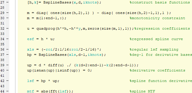
BsplineBases is a wrapper for the C function in Dr. de Leeuw’s paper, which constructs spline basis functions $\texttt{h}$ = $h$ recursively per de Boor. Quadprog solves for coefficients $\texttt{u}$ = $\hat{u}$ by monotone regression (lsqlin gives the same results but it is slower). And $\texttt{up}$ = $\hat{u}'$ is the result of Dr. Shene’s algebraic calculation of derivative coefficients shown earlier, this time vectorized.

Alternatively one could replace lines 29-32 above by the normal equation (simply $\texttt{u = h} \; \backslash \; \texttt{y}$ ), thus abandoning monotonicity and obtaining a normal B-Spline regression with the same (or a suitably tailored) knot vector.

That’s all that is needed to go from the projected raw edge intensity data set ( $x_i,y_i$ ) to ESF, LSF and MTF by expressing the ESF as a B-Spline function. It will work with a handful of pixels on either side of the edge but for better resolution and accuracy I prefer 16 or 32, controlled by the constant $\texttt{roi}$ . A link to the Matlab code can be found in the notes.^[10]

Appendix II: Parameters and Limitations

Given a projected edge raw data set there are only two parameters required to obtain the spline functions that lead to the MTF estimate for the imaging system:

B-Spline degree; and
knot position vector.

I determined both empirically for my own photographic purposes: back-lit utility knives captured in the raw data by enthusiast-level digital cameras with pixels around 3-6 $\mu m$ and decent lenses at typical working f-numbers near the center of the image. Though they work well off-center with smaller pixels and printed edges too.

Figure 13. Fuji GFX50s 110mm/2.8 at f/2.8, raw razor edge captured by Jim Kasson. Pixel pitch is about 5.33um.

In fact the minimalist monotonic approach works well in most imaging situations with quartic B-Splines for the ESF and a dozen knots evenly sprinkled over the edge transition, my default choice for the two parameters.

By the interaction of the given spline degree with the diffraction extinction spatial frequency of the lens we can additionally set a rough minimum knot density requirement across the edge transition. A quartic ESF means a cubic LSF, in which case the requirement across the edge is at least this many knots per pixel (k/p)

$\begin{equation*} Knot Density (cubic) > \approx 3 \cdot \frac{p}{N}, \; \text{k/p} \end{equation*}$

as a function of pixel pitch ( $p$ ) in microns and the effective f-number of the lens ( $N$ ). More generally, as explained in Appendix III, spline degree and knot spans set an upper bound on the spatial frequencies possible within the LSF spline function as shown below for a sensor with a 4.35um pitch:

Figure 14. For edges captured by a camera with a 4.35um pitch and f-number on the y axis, choose the next knot density up at the desired spline degree. For instance for an f/1.4 capture use an LSF of degree 1 and 8 k/p, degree 2 and 9 k/p or degree 3 and 10 k/p (my choice). For an f/4 capture there are more options. Vice versa, for a given degree and knot density, read the minimum allowable f-number on the y-axis. This figure is extracted from Figure 28.

As long as they are not off to left field, the resulting curves are surprisingly insensitive to their choice. For instance below the f/2.8 capture of Figure 13 achieves very similar results with LSF spline degrees from 1 to 10 and the approximate knot density suggested by Figure 14 or 28 (one up from the intersection of capture f-number and the chosen degree):

Same SFR, different B-Spline parameters for the LSF. The blue curve is the result of parameters chosen automatically: a dozen knots over the edge transition.

To limit the number of variables and keep things easy to follow, regressions in this page were based on cubic spline LSFs and simple knots were mostly set at a fixed rate of 4 per pixel (pitch) around the transition. Based on the formula and Figure above this knot density is greater than the minimum for the f/4+ f-numbers used with Nikon cameras in these plots – but not necessarily for the GFX50s above.

In my typical testing conditions there are normally only shallow waves in the ESF after the transition, say from about 3 pixels from the center of the edge, so knot distance can easily be doubled or more from then on, and I do.

Figure 15. From printed slanted edge captured by DPReview in raw file 2099 by a Nikon Z7 with 85mm/1.8G at f/5.6. The printed edge is burdened with its own MTF, which is convolved with the imaging system’s. With a knife edge and good technique we would expect MTF50 greater than 0.4 c/p with this setup.

It is good practice in spline theory to use the least number of knots necessary, thus limiting high frequency noise for reasons explained in the next section. Without information about the imaging system, my preferred method is a quartic degree and knots spaced automatically so that there are about a dozen over the ESF transition, then double the span for the next five knots, double it again for the next five, completing the sequence with a knot at every other pixel.^[9] This way my edges typically require less than 50 knots, with 3-6 knots per pixel around the transition as you can see from the figures and attached Matlab code.

Too few knots limit the higher frequencies but too many can have the splines trying a fit to the noise. With my default parameters there is often some overfitting around the upper shoulder due to the sharp bend and inevitable increased noise there, though the effect is mild and well controlled by the monotonicity constraint. However, approaching 10 knots per pixel, my limit, the potential for overfitting increases, as shown in the LSF of the following low-contrast simulated capture:

Figure 16. With my parameters I often see some overfitting in the upper shoulder due to a sharp bend in combination with increased noise, though it does not seem to affect the final SFR much in practice. Effective pixel aperture in this simulated example was 3.8um.

Given the larger standard deviation of noise in the bright portion of the projected raw data compared to the darker part, one might be tempted to assign different weights to each of them. Or to run two regressions, one each for the dark and bright portions, but in light testing I did not see any tangible improvement in the results. Weighted and unweighted also appear to produce very similar results with PAVA.

Figure 17. GFX50s with Otus 85mm at f/4, raw razor capture by Jim Kasson.

This is all empirical and I am sure the number of knots could be pared down significantly by measuring the effect of various knot spacings away from the transition. Eliminating overfitting around the upper shoulder and reducing the number of knots away from it would be an interesting line of further inquiry, though I have not pursued it because the described strategy works well as-is with my raw edges, producing results practically indistinguishable from MTF Mapper’s.

Some edge angles result in projected $x_i$ that bunch up, leaving large empty areas where the monotonic regressed ESF may be forced to slow down, creating an unsightly LSF with high frequency noise. The issue generally does not present itself with the proposed knot spans.

Figure 18. Bad edge angles cause projected raw intensities to collect at fewer, discrete regular distances.

The Nikon D610 has a relatively strong two-dot Antialiasing filter active only in the horizontal direction, as seen in the null it causes below:

Figure 19. Nikon D610 200mm/4 at f/8, Anti-Aliasing filter forces a null around 0.65 c/p horizontally, note the change of scale.

Diffraction at f/22 with a 0.595um pitch means light should result in diffraction extinction and no energy above 0.5 c/p:

Figure 20. Razor edge captured by Nikon D610 50mm/1.8G at f/22 with diffraction extinction at 0.5 c/p.

Clearly the degree and knot spacing interact. A degree of zero means that the function within each simple knot span is a constant, hence the regression creates discontinuous steps; a degree of one connects each knot to the next in a straight line, similar to the naive approach; with a degree of two the function is piecewise quadratic; at three it is cubic and when it looks like it is not straining to follow the physical line spread profile.

So since the LSF is the derivative of the ESF, I chose a degree of 4, quartic, for ESF splines, so that the LSF would be made up of cubic splines. This works well with the edges I analyze and I have not felt the need to go higher. Though one could, while keeping an eye on Figure 28.

The monotonicity criterion can also affect the ESF, though mildly. As mentioned I chose to ensure that B-Spline regression results in increasing coefficients, which Dr. de Leeuw suggests is equivalent to fitting I-Splines in Section 4.2 of his paper. One could also use increasing values in the resulting curve as a criterion (section 4.3) but I have verified that it results in slightly more overfitting while being more expensive in terms of CPU cycles.

In the end, unless one needs to understand every step along the way or roll one’s own, open source MTF Mapper is the easier, more well rounded tool to use – the best and most professional out there. Here we simply provided some hopefully easy to understand and intuitive validation of its results, front-loading all uncertainty to the estimation of a physically-relevant, well-behaved, robust, ESF.

Appendix III – The Spectrum of B-Spline Functions

As one can gather from Dr. de Leeuw’s working paper, B-spline basis functions are computed recursively per de Boor, effectively convolving a square pulse the length of a knot span with itself repeatedly, one top hat convolution for every degree of the spline. They therefore have local, compact support, their extent in knots equal to the spline’s order (degree + 1), as shown below:

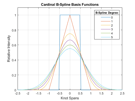
Figure 22. Cardinal B-Splines of the shown degree obtained by repeated convolution with the spline of degree 0, a top hat.

ESF spline functions generated by the method discussed in this article are a linear combination of B-spline basis functions $h$ . In the simplest case of infinitely many uniformly spaced knots (cardinal B-Splines), the basis functions are all of similar shape though their range of influence on the final spline function is shifted to match the position of the knots they apply to, per the definition in earlier Equations 1-3.

Figure 23. Central knots with corresponding active area of B-Spline Basis Function of degree 4.

Coefficients $u$ are then simply the weights associated with each shifted B-Spline and ESF = $h*u$ ; the same is true of LSF basis functions of one degree less $h'$ and their coefficients $\hat{u}'$ so LSF = $h'*\hat{u}'$ , as previously discussed.

Since the resulting spline function is a linear combination of phase-shifted B-Splines, if we know the bandwidth of the B-Splines we also know the bandwidth of the spline function. The bandwidth of the basis functions is surprisingly easy to calculate, because the Fourier Transform of a top hat in the spatial domain becomes a normalized sinc function in the frequency domain and convolutions in one are multiplications in the other, so the spectrum of the basis functions is simply

(8) $\begin{equation*} H(f) = \Big|\frac{sin(\pi f)}{\pi f}\Big|^{d+1} \end{equation*}$

with $f$ the spatial frequency and $d$ the degree of the B-splines, at least in the cardinal case around the edge transition that I am using to make the point. As we know sinc functions have infinite support, meaning that they continue on forever. This reminds us that we cannot have a time and bandwidth limited signal at the same time, per the Uncertainty Principle applied to Time-Frequency Duality. So either we come up with basis functions with pretend-infinite support or we cannot band limit them. Why does Lancsos come to mind?

Fortunately that is not necessary because raising a sinc to a power tends to emphasize the much larger central pulse at the expense of the harmonics so this is what the spectra of B-Splines of different degree look like after normalization:

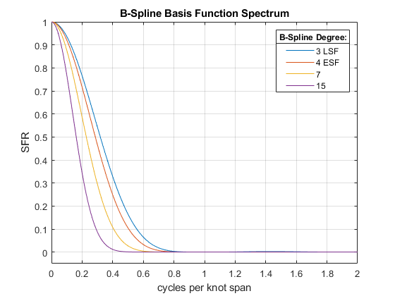
Figure 24. Spectra of the Cardinal B-Splines of the shown degree. They set an upper limit to the spatial frequencies that can be present in a spline function of the given degree.

Our cubic LSF (blue curve) appears practically band limited once normalized, with virtually no relative energy above about 3/4 cycles per knot span (c/k). The knot density around the edge in the examples in this page is mostly set at 4 knots per pixel (k/p), so the B-spline basis functions could generate spatial frequencies all the way out to about 3/4 * 4 = 3 cycles per pixel pitch (c/p), see how the units play out. This is plenty for my typical measurements.

In particular, if we set up the monotone fit for the ESF with quartic splines, the LSF from which MTF is derived will be cubic and so the relevant B-Spline spectrum is $sinc^4$ per Equation (8), representing the gamut of allowed frequencies in the LSF spline function. Here is the effect of different knot spans on the frequency response of a cubic LSF, expressed as a function of the sensor’s pixel pitch to be consistent with the other plots (c/k curve * k/p = c/p curve):

Figure 25. Spectrum of cubic B-Spline basis functions with knots spaced at the shown knot per pixel density (k/p), spatial frequency in cycles per pixel.

The cubic LSF blue curve of Figure 24 is scaled by different knot densities in the above plot. In other words, if we believe that the 3 k/p curve (yellow here) is usable down to, say, 5% of its strength this effective cubic spline frequency limit will simply scale linearly with knot density $kd$

(9) $\begin{equation*} \text{Band Limit(d=3)}_{kd} \approx 1.9 \cdot \frac{kd}{3}, \; \text{c/p} \end{equation*}$

because the relative 3 k/p SFR curve hits 5% at a spatial frequency of 1.87 c/p, see Figure 29 at bottom for thresholds at other densities. I chose 5% instead of less to keep a, possibly unnecessary, safety margin (anyone?). We can compare this frequency limitation with theoretical diffraction extinction for a photographic lens with circular aperture

(10) $\begin{equation*} \text{Band Limit}_{diff} \approx \frac{p}{\lambda N}, \; \text{c/p} \end{equation*}$

with pixel pitch $p$ and mean light wavelength $\lambda$ in microns, and $N$ the effective f-number of the lens. In this case the approximate sign is there to indicate that often $\lambda$ and $N$ are not known precisely. Equating the two and solving for $kd$ we can obtain an approximate, rough minimum knot density for cubic splines. Assuming 0.535um as the typical mean wavelength in the green channel of current Bayer sensors

(11) $\begin{equation*} \text{Knot Density(d=3)}_{\lambda} > \approx 3 \cdot \frac{p}{N}, \; \text{k/p} \end{equation*}$

Minimum knot density ( $kd$ ) is in knots per pixel, with pixel pitch $p$ in microns and $N$ the effective f-number of the lens. Note that for a given camera, minimum knot density increases quickly with smaller f-numbers.

For example, with the 4.35 um pitch of a Nikon Z7 at f/4, minimum knot density would be 3.3 knots per pixel. A cubic LSF with 2 knots per pixel around the edge transition (the orange curve in Figure 25 above) would not cut it because it only allows frequencies below 1.5 c/p through, too tight for a Z7 as setup, with diffraction extinction out at about 2/cp per Equation (10). The 3 knots per pixel yellow curve there appears to be able to supply energy close to extinction and in fact its MTF looks good almost to the end, as shown below. 4 k/p would leave a little margin and be better still.

Figure 26. MTF obtained from a simulated slanted edge equivalent to a Nikon Z7 with Z 50mm/1.8 S at f/4 in the center. The ESF was determined by quartic B-Spline regression, resulting in a Cubic B-Spline LSF. MTF curves are shown for knots placed at 6 per pixel and 3 per pixel around the transition. Results are virtually identical other than a slight loss of energy beyond 1.8 c/p at 3 knots per pixel.

We can use Equation (9) or Figure 14 or 28 to determine the band limit imposed by a given knot density on a cubic spline. The plot below refers to a capture by a Nikon Z7 with a 4.35um pixel at f/11 that should have no energy above about 0.75 c/p because of diffraction extinction, as we approximately see. At 3 k/p (chosen by the dozen-knots-over-transition algorithm) there is some residual energy hovering beyond it, indicating high frequency noise. And in fact Equation (9) indicates a band limit due to knot density only at around 1.9 c/p, which we approximately see in the blue curve.

Figure 27 Nikon Z7 at f/11. The blue curve from cubic LSF splines and 3 knots per pixel shows noisy energy above diffraction extinction at about 3/4 c/p. The dotted curve was obtained by applying Equation (11) with a bit of a margin at 1.5 k/p, effectively band limiting the result to around 1 c/p.

However, the minimum knot density suggested by Equation (11) is 1.2 k/p, meaning that we could use fewer knots for the same result helping to keep high frequency noise in check. The dotted curve was obtained at 1.5 knots/pixel. It follows its 3 k/p predecessor faithfully though limiting spatial frequencies to about 1 c/p, thus abating residual noise beyond it.

Typical cameras in digital photography tend to have pixel pitches around 4 micrometers and consumer lenses often are at their sharpest around f/5. This suggests diffraction extinction in such testing conditions around 1.5 c/p. In such a generic case, with a cubic spline LSF, one could not be faulted for using 3 knots per pixel around the edge based on the Figures below. That is of course not the case with high-end primes that can be used at lower f-numbers.

So knot span and spline degree can indeed be balanced with diffraction extinction to ensure that only legitimate frequencies are present and/or to help control high frequency noise. I didn’t explicitly do that with the recommended cubic LSF and knot placing strategy, I just checked that there was plenty of bandwidth to go around in typical testing conditions, and there was (with a couple of notable exceptions).

On the other hand the recommended strategy of a dozen knots over the transition is conservative and takes all this figuring out of the equation. In the end it makes little difference in practice as mentioned.

Anyways, this strays way off the minimalist track so I will stop here. Should you pursue it further, let me know what parameter combinations work best for your use cases.

Figure 28. Threshold spatial frequency in cycles per pixel beyond which a B-spline basis function of the given degree and knot density (in knots per pixel, k/p) will provide energy at less than 5% of its potential. With a known pixel pitch the y-axis can be expressed as an f-number per Equation (10), see Figure 14.

Figure 29. Threshold spatial frequency in cycles per pixel beyond which the given knot density with a cubic B-Spline function provides less than 5% of potential energy.

Notes and References

_{1. Frans van den Berg’s excellent open source MTF Mapper determines the ESF, LSF, SFR/MTF of your camera and lens by capturing slanted edges at home. It is robust and comes with an easy to use graphical user interface. I would like to thank Frans for his help and guidance in this journey of discovery.

2. Slanted-Edge MTF for Digital Camera and Scanner Analysis, Peter D. Burns, Eastman Kodak Company, 2000.

3. sfrmat5 is used in Version 4 of ISO standard 12233 for edge-based camera resolution evaluation, which was published on Feb 17, 2023. It can be downloaded from here.

4. Exceedingly Simple Monotone Regression, Jan de Leeuw, 2017.

5. lsqisotonic is a fast implementation of the Pool Adjacent Violators algorithm in Matlab as modified by Yun Wang, 2017. I believe this version is in the open domain and does not require a toolbox.

6. Computing and Fitting Monotone Splines, Jan de Leeuw, 2017.

7. Derivative of a B-Spline Curve, Dr. Ching-Kuang Shene, 2014. My notation differs from Dr. Shene’s to be closer to de Leeuw’s: my u’=up is his Qi, my d his p, my knots=k are his ui and my original regressed coefficients=u are his Pi.

8. Although being able to obtain the derivative semi-analytically is intellectually stimulating and comforting, taking finite differences of unregularized ESF spline data actually results in virtually indistinguishable LSF results because of the often quasi-random, massively oversampled curve. At least we know that’s the case.

9. For another automatic knot selection strategy see: Knot calculation for spline fitting via sparse optimization, Kongmei Kang et. al. 2015.

10. The Matlab function used to perform the monotonic PAVA and Spline regressions in this page on projected raw edge data, and a few data set examples, can be downloaded by clicking here.}

Strolls with my Dog